Natural and artificial perturbations

from matplotlib import pyplot as plt
import numpy as np

from astropy.coordinates import solar_system_ephemeris
from astropy.time import Time, TimeDelta
from astropy import units as u

from poliastro.bodies import Earth, Moon
from poliastro.constants import rho0_earth, H0_earth

from poliastro.core.elements import rv2coe
from poliastro.core.perturbations import (
    atmospheric_drag_exponential,
    third_body,
    J2_perturbation,
)
from poliastro.core.propagation import func_twobody
from poliastro.ephem import build_ephem_interpolant
from poliastro.plotting import OrbitPlotter3D
from poliastro.twobody import Orbit
from poliastro.twobody.propagation import CowellPropagator
from poliastro.twobody.sampling import EpochsArray
from poliastro.util import norm

# More info: https://plotly.com/python/renderers/
import plotly.io as pio

pio.renderers.default = "plotly_mimetype+notebook_connected"

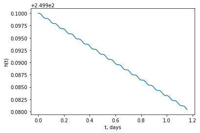
Atmospheric drag

The poliastro package now has several commonly used natural perturbations. One of them is atmospheric drag! See how one can monitor decay of the near-Earth orbit over time using our new module poliastro.twobody.perturbations!

R = Earth.R.to(u.km).value
k = Earth.k.to(u.km**3 / u.s**2).value

orbit = Orbit.circular(
    Earth, 250 * u.km, epoch=Time(0.0, format="jd", scale="tdb")
)

# parameters of a body
C_D = 2.2  # dimentionless (any value would do)
A_over_m = ((np.pi / 4.0) * (u.m**2) / (100 * u.kg)).to_value(
    u.km**2 / u.kg
)  # km^2/kg
B = C_D * A_over_m

# parameters of the atmosphere
rho0 = rho0_earth.to(u.kg / u.km**3).value  # kg/km^3
H0 = H0_earth.to(u.km).value

tofs = TimeDelta(np.linspace(0 * u.h, 100000 * u.s, num=2000))


def f(t0, state, k):
    du_kep = func_twobody(t0, state, k)
    ax, ay, az = atmospheric_drag_exponential(
        t0,
        state,
        k,
        R=R,
        C_D=C_D,
        A_over_m=A_over_m,
        H0=H0,
        rho0=rho0,
    )
    du_ad = np.array([0, 0, 0, ax, ay, az])

    return du_kep + du_ad


rr, _ = orbit.to_ephem(
    EpochsArray(orbit.epoch + tofs, method=CowellPropagator(f=f)),
).rv()

plt.ylabel("h(t)")
plt.xlabel("t, days")
plt.plot(tofs.value, norm(rr, axis=1) - Earth.R)

[<matplotlib.lines.Line2D at 0x7fe9e030f4f0>]

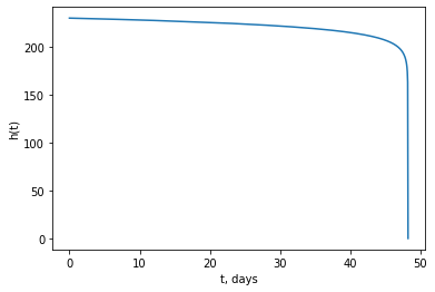
Orbital Decay

If atmospheric drag causes the orbit to fully decay, additional code is needed to stop the integration when the satellite reaches the surface.

Please note that you will likely want to use a more sophisticated atmosphere model than the one in atmospheric_drag for these sorts of computations.

from poliastro.twobody.events import LithobrakeEvent

orbit = Orbit.circular(
    Earth, 230 * u.km, epoch=Time(0.0, format="jd", scale="tdb")
)
tofs = TimeDelta(np.linspace(0 * u.h, 100 * u.d, num=2000))

lithobrake_event = LithobrakeEvent(R)
events = [lithobrake_event]

rr, _ = orbit.to_ephem(
    EpochsArray(
        orbit.epoch + tofs, method=CowellPropagator(f=f, events=events)
    ),
).rv()

print(
    "orbital decay seen after", lithobrake_event.last_t.to(u.d).value, "days"
)

orbital decay seen after 48.217988400734775 days

plt.ylabel("h(t)")
plt.xlabel("t, days")
plt.plot(tofs[: len(rr)].value, norm(rr, axis=1) - Earth.R)

[<matplotlib.lines.Line2D at 0x7fe9e03be700>]

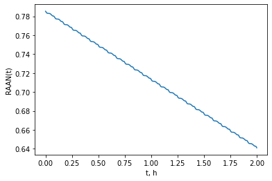
Evolution of RAAN due to the J2 perturbation

We can also see how the J2 perturbation changes RAAN over time!

r0 = np.array([-2384.46, 5729.01, 3050.46]) * u.km
v0 = np.array([-7.36138, -2.98997, 1.64354]) * u.km / u.s

orbit = Orbit.from_vectors(Earth, r0, v0)

tofs = TimeDelta(np.linspace(0, 48.0 * u.h, num=2000))


def f(t0, state, k):
    du_kep = func_twobody(t0, state, k)
    ax, ay, az = J2_perturbation(
        t0, state, k, J2=Earth.J2.value, R=Earth.R.to(u.km).value
    )
    du_ad = np.array([0, 0, 0, ax, ay, az])

    return du_kep + du_ad


rr, vv = orbit.to_ephem(
    EpochsArray(orbit.epoch + tofs, method=CowellPropagator(f=f)),
).rv()

# This will be easier to compute when this is solved:
# https://github.com/poliastro/poliastro/issues/380
raans = [
    rv2coe(k, r, v)[3]
    for r, v in zip(rr.to_value(u.km), vv.to_value(u.km / u.s))
]

plt.ylabel("RAAN(t)")
plt.xlabel("t, h")
plt.plot(tofs.value, raans)

[<matplotlib.lines.Line2D at 0x7fe9db698eb0>]

3rd body

Apart from time-independent perturbations such as atmospheric drag, J2/J3, we have time-dependent perturbations. Let’s see how the Moon changes the orbit of GEO satellite over time!

# database keeping positions of bodies in Solar system over time
solar_system_ephemeris.set("de432s")

epoch = Time(
    2454283.0, format="jd", scale="tdb"
)  # setting the exact event date is important

# create interpolant of 3rd body coordinates (calling in on every iteration will be just too slow)
body_r = build_ephem_interpolant(
    Moon,
    28 * u.day,
    (epoch.value * u.day, epoch.value * u.day + 60 * u.day),
    rtol=1e-2,
)

initial = Orbit.from_classical(
    Earth,
    42164.0 * u.km,
    0.0001 * u.one,
    1 * u.deg,
    0.0 * u.deg,
    0.0 * u.deg,
    0.0 * u.rad,
    epoch=epoch,
)

tofs = TimeDelta(np.linspace(0, 60 * u.day, num=1000))


def f(t0, state, k):
    du_kep = func_twobody(t0, state, k)
    ax, ay, az = third_body(
        t0,
        state,
        k,
        k_third=400 * Moon.k.to(u.km**3 / u.s**2).value,
        perturbation_body=body_r,
    )
    du_ad = np.array([0, 0, 0, ax, ay, az])

    return du_kep + du_ad


# multiply Moon gravity by 400 so that effect is visible :)
ephem = initial.to_ephem(
    EpochsArray(initial.epoch + tofs, method=CowellPropagator(rtol=1e-6, f=f)),
)

frame = OrbitPlotter3D()

frame.set_attractor(Earth)
frame.plot_ephem(ephem, label="orbit influenced by Moon")

Applying thrust

Apart from natural perturbations, there are artificial thrusts aimed at intentional change of orbit parameters. One of such changes is simultaneous change of eccentricity and inclination:

from poliastro.twobody.thrust import change_ecc_inc

ecc_0, ecc_f = 0.4, 0.0
a = 42164  # km
inc_0 = 0.0  # rad, baseline
inc_f = 20.0 * u.deg
argp = 0.0  # rad, the method is efficient for 0 and 180
f = 2.4e-6 * (u.km / u.s**2)

k = Earth.k.to(u.km**3 / u.s**2).value
orb0 = Orbit.from_classical(
    Earth,
    a * u.km,
    ecc_0 * u.one,
    inc_0 * u.deg,
    0 * u.deg,
    argp * u.deg,
    0 * u.deg,
    epoch=Time(0, format="jd", scale="tdb"),
)

a_d, _, t_f = change_ecc_inc(orb0, ecc_f, inc_f, f)


def f(t0, state, k):
    du_kep = func_twobody(t0, state, k)
    ax, ay, az = a_d(
        t0,
        state,
        k,
    )
    du_ad = np.array([0, 0, 0, ax, ay, az])

    return du_kep + du_ad


tofs = TimeDelta(np.linspace(0, t_f, num=1000))

ephem2 = orb0.to_ephem(
    EpochsArray(orb0.epoch + tofs, method=CowellPropagator(rtol=1e-6, f=f)),
)

frame = OrbitPlotter3D()

frame.set_attractor(Earth)
frame.plot_ephem(ephem2, label="orbit with artificial thrust")

Combining multiple perturbations

It might be of interest to determine what effect multiple perturbations have on a single object. In order to add multiple perturbations we can create a custom function that adds them up:

from numba import njit as jit

# Add @jit for speed!
@jit
def a_d(t0, state, k, J2, R, C_D, A_over_m, H0, rho0):
    return J2_perturbation(t0, state, k, J2, R) + atmospheric_drag_exponential(
        t0, state, k, R, C_D, A_over_m, H0, rho0
    )

# propagation times of flight and orbit
tofs = TimeDelta(np.linspace(0, 10 * u.day, num=10 * 500))
orbit = Orbit.circular(Earth, 250 * u.km)  # recall orbit from drag example


def f(t0, state, k):
    du_kep = func_twobody(t0, state, k)
    ax, ay, az = a_d(
        t0,
        state,
        k,
        R=R,
        C_D=C_D,
        A_over_m=A_over_m,
        H0=H0,
        rho0=rho0,
        J2=Earth.J2.value,
    )
    du_ad = np.array([0, 0, 0, ax, ay, az])

    return du_kep + du_ad


# propagate with J2 and atmospheric drag
rr3, _ = orbit.to_ephem(
    EpochsArray(orbit.epoch + tofs, method=CowellPropagator(f=f)),
).rv()


def f(t0, state, k):
    du_kep = func_twobody(t0, state, k)
    ax, ay, az = atmospheric_drag_exponential(
        t0,
        state,
        k,
        R=R,
        C_D=C_D,
        A_over_m=A_over_m,
        H0=H0,
        rho0=rho0,
    )
    du_ad = np.array([0, 0, 0, ax, ay, az])

    return du_kep + du_ad


# propagate with only atmospheric drag
rr4, _ = orbit.to_ephem(
    EpochsArray(orbit.epoch + tofs, method=CowellPropagator(f=f)),
).rv()

fig, (axes1, axes2) = plt.subplots(nrows=2, sharex=True, figsize=(15, 6))

axes1.plot(tofs.value, norm(rr3, axis=1) - Earth.R)
axes1.set_ylabel("h(t)")
axes1.set_xlabel("t, days")
axes1.set_ylim([225, 251])

axes2.plot(tofs.value, norm(rr4, axis=1) - Earth.R)
axes2.set_ylabel("h(t)")
axes2.set_xlabel("t, days")
axes2.set_ylim([225, 251])

(225.0, 251.0)

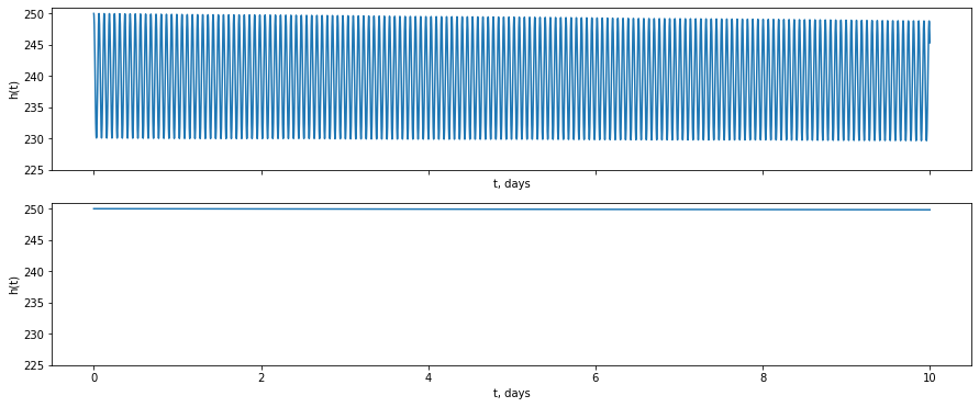
The first plot shows the altitude of the orbit changing due to both atmospheric drag and the J2 effect, the second plot shows only the effect of atmospheric drag.