New Horizons launch and trajectory

Main data source: Guo & Farquhar “New Horizons Mission Design” http://www.boulder.swri.edu/pkb/ssr/ssr-mission-design.pdf

from astropy import time
from astropy import units as u

from poliastro import iod

from poliastro.bodies import Sun, Earth, Jupiter
from poliastro.ephem import Ephem
from poliastro.frames import Planes
from poliastro.plotting import StaticOrbitPlotter
from poliastro.twobody import Orbit
from poliastro.util import norm

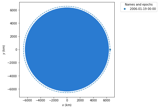
Parking orbit

Quoting from “New Horizons Mission Design”:

It was first inserted into an elliptical Earth parking orbit of perigee altitude 165 km and apogee altitude 215 km. [Emphasis mine]

r_p = Earth.R + 165 * u.km
r_a = Earth.R + 215 * u.km

a_parking = (r_p + r_a) / 2
ecc_parking = 1 - r_p / a_parking

parking = Orbit.from_classical(
    Earth,
    a_parking,
    ecc_parking,
    0 * u.deg,
    0 * u.deg,
    0 * u.deg,
    0 * u.deg,  # We don't mind
    time.Time("2006-01-19", scale="utc"),
)

print(parking.v)
parking.plot()

[0.         7.81989358 0.        ] km / s

[<matplotlib.lines.Line2D at 0x7f31c1362280>,
 <matplotlib.lines.Line2D at 0x7f31c1362e20>]

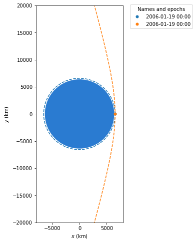
Hyperbolic exit

Hyperbolic excess velocity:

\[v_{\infty}^2 = \frac{\mu}{-a} = 2 \varepsilon = C_3\]

Relation between orbital velocity \(v\), local escape velocity \(v_e\) and hyperbolic excess velocity \(v_{\infty}\):

\[v^2 = v_e^2 + v_{\infty}^2\]

Option a): Insert \(C_3\) from report, check \(v_e\) at parking perigee:

C_3_A = 157.6561 * u.km**2 / u.s**2  # Designed

a_exit = -(Earth.k / C_3_A).to(u.km)
ecc_exit = 1 - r_p / a_exit

exit = Orbit.from_classical(
    Earth,
    a_exit,
    ecc_exit,
    0 * u.deg,
    0 * u.deg,
    0 * u.deg,
    0 * u.deg,  # We don't mind
    time.Time("2006-01-19", scale="utc"),
)

norm(exit.v).to(u.km / u.s)

$16.718069 \; \mathrm{\frac{km}{s}}$

Quoting “New Horizons Mission Design”:

After a short coast in the parking orbit, the spacecraft was then injected into the desired heliocentric orbit by the Centaur second stage and Star 48B third stage. At the Star 48B burnout, the New Horizons spacecraft reached the highest Earth departure speed, estimated at 16.2 km/s, becoming the fastest spacecraft ever launched from Earth. [Emphasis mine]

v_estimated = 16.2 * u.km / u.s

print(
    "Relative error of {:.2f} %".format(
        (norm(exit.v) - v_estimated) / v_estimated * 100
    )
)

Relative error of 3.20 %

So it stays within the same order of magnitude. Which is reasonable, because real life burns are not instantaneous.

from matplotlib import pyplot as plt

fig, ax = plt.subplots(figsize=(8, 8))
op = StaticOrbitPlotter(ax=ax)

op.plot(parking)
op.plot(exit)

ax.set_xlim(-8000, 8000)
ax.set_ylim(-20000, 20000)

(-20000.0, 20000.0)

Option b): Compute \(v_{\infty}\) using the Jupyter flyby

According to Wikipedia, the closest approach occurred at 05:43:40 UTC. We can use this data to compute the solution of the Lambert problem between the Earth and Jupiter:

nh_date = time.Time("2006-01-19 19:00", scale="utc").tdb
nh_flyby_date = time.Time("2007-02-28 05:43:40", scale="utc").tdb
nh_tof = nh_flyby_date - nh_date

nh_r_0, v_earth = Ephem.from_body(Earth, nh_date).rv(nh_date)
nh_r_f, v_jup = Ephem.from_body(Jupiter, nh_flyby_date).rv(nh_flyby_date)

nh_v_0, nh_v_f = iod.lambert(Sun.k, nh_r_0, nh_r_f, nh_tof)

The hyperbolic excess velocity is measured with respect to the Earth:

C_3_lambert = (norm(nh_v_0 - v_earth)).to(u.km / u.s) ** 2
C_3_lambert

$158.45628 \; \mathrm{\frac{km^{2}}{s^{2}}}$

print("Relative error of {:.2f} %".format((C_3_lambert - C_3_A) / C_3_A * 100))

Relative error of 0.51 %

Which again, stays within the same order of magnitude of the figure given to the Guo & Farquhar report.

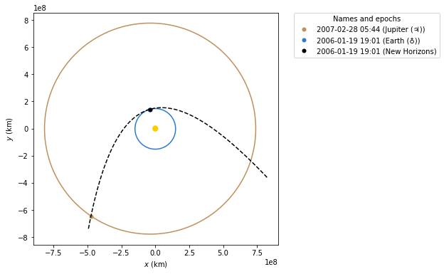
From Earth to Jupiter

nh = Orbit.from_vectors(Sun, nh_r_0, nh_v_0, nh_date)

op = StaticOrbitPlotter(plane=Planes.EARTH_ECLIPTIC)

op.plot_body_orbit(Jupiter, nh_flyby_date)
op.plot_body_orbit(Earth, nh_date)

op.plot(nh, label="New Horizons", color="k")

[<matplotlib.lines.Line2D at 0x7f31c06e49a0>,
 <matplotlib.lines.Line2D at 0x7f31c06e41f0>]