Multiple revolutions on Lambert’s problem
After the implementation of Izzo’s algorithm in poliastro, it is possible to solve the Lambert’s problem within the multi-revolution scenario. Before introducing the usage of this feature, let us remember what is the Lambert’s problem and explain some of the misconceptions behind the problem.
Review of Lambert’s problem scenarios
The Lambert’s problem tries to solve for the orbit which passes trhough \(\vec{r_{0}}\) and \(\vec{r_{f}}\) being knwon the time of flight \(\Delta t\) between these two positions. It is, in fact, the boundary value problem (BVP) of the two body problem.
There are two scenarios for solving Lambert’s problem:
Single revolution or direct-transfer arc. This type of solution considers transfer angles which do not exceed \(360\) degrees. Elliptic, parabolic and hyperbolic transfer solutions can be found within this scenario.
Multiple revolution arc. This second case asumes transfer angles which exceed a single revolution (i.e. \(>360\) degrees). Because multiple revolutions are required, transfer solutions need to be closed orbit and therefore, only elliptical orbits can be found in this scenario.
Any Lambert’s problem solver in the form of a computer algorithm must accept at least the following parameters:
The gravitational parameter \(k\), that is the mass of the attracting body times the gravitational constant.
Initial position vector \(\vec{r_0}\).
Final position vector \(\vec{r}\).
Time of flight between initial and final vectors \(\Delta t\).
Number of desired revolutions \(M\).
Type of transfer orbit: prograde or retrograde.
Type of path (only for multi-revolution scenario): low or high.
Maximum number of iterations and allowed numerical tolerances.
Misconceptions about Lambert’s problem
The literature about Lambert’s problem is abundant. However, some misconceptions have arise during the last years as the problem has become more and more popular due to its aplications. Here, some of those misconceptions are presented and explained.
Type of transfer orbit: prograde or retrograde
The transfer angle \(\Delta \theta\) between \(\vec{r_0}\) and \(\vec{r}\) position vectors plays a vital role in the problem. However, notice that \(\Delta \theta\) is not an input of the problem. In fact, its vlaue needs to be computed using:
The arccos function will return always the shortest angle between both position vectors. Therefore, what happens with transfer angles \(180 < \Delta \theta < 360\)? In this case, a boolean is required to correct the value of the transfer angle. In poliastro this variable is named is_prograde and it controls the value of the transfer angle such that:
When
is_prograde=True, solution orbit has an inclination less than \(\text{inc} < 180\) degrees (prograde orbit).Otherwise, when
is_prograde=False, solution orbit inclination has \(\text{inc} > 180\) degrees (retrograde orbit.)
Type of transfer path: low or high
The type of path is a boolean variable which allows the user to filter out the solution when two of them are found. Multiple solutions only appear in the multi-revolution case. The geometry of this scenario is presented in the figure below:
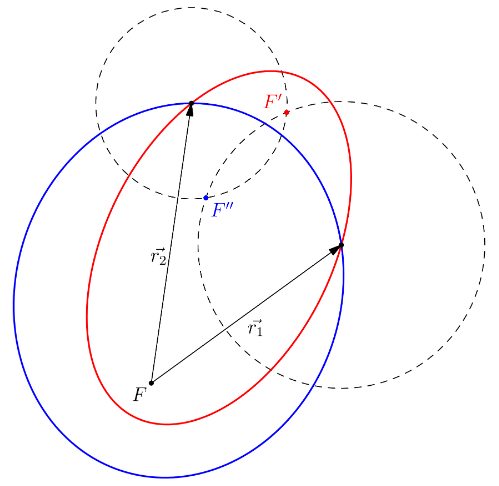
Notice there are a total of two orbits (red and blue) connecting the position vectors \(\vec{r_1}\) to \(\vec{r_2}\). A total of four solutions are found:
Red orbit (high path) prograde.
Red orbit (high path) retrograde.
Blue orbit (low path) prograde.
Blue orbit (low path) retrograde.
The type of path allows to select the orbit whose second focus is located above (high) or below (low) the chord line. The chord line is the line connecting the initial and final position vectors and can be computed as \(\vec{c} = \vec{r} - \vec{r_0}\).
Then, what is short/long path?
In the popular book by Bate&Mueller named “Fundamentals of astrodynamics” it was introduced this misconception and Vallado also adopted it in his “Fundamentals of astrodynamics and applications”, where he reproduces the original figure by Bate&Mueller.
These authors use the terms “long” and “short” paths to control the transfer angle value, as mentioned previously. It is better to use the terms “prograde” or “retrograde” instead.
Because previous cited volumes are very popular and considered reference materials in the subject, this would explain the huge missconception about previous terms and their purpose within Lambert’s problem solvers.
A note on the minimum energy transfer orbit
The minimum energy transfer orbit is the particular orbit which exhibits the lowest characteristic energy when performing the transfer between \(\vec{r_0}\) and \(\vec{r}\) position vectors.
However, notice this orbit is only possible for a particular transfer time named \(\Delta t_{\text{min}}\), which might be greater or lower than the current desired time of flight \(\Delta t\).
The minimum energy transfer orbit is used as a reference point by Lambert’s problem solvers when carrying out the iterative method for computing the solution.
Exploring the single and multi-revolution scenarios using poliastro
Now, let us present how to use poliastro to solve for the multiple revolutions scenario. The idea is to compute all possible transfer orbits between Earth and Mars. Therefore, we need first to compute the initial position of the Earth and the final position of times for a given desired amount of time.
[1]:
from astropy import units as u
from astropy.time import Time

from poliastro.bodies import Sun, Earth, Mars
from poliastro.ephem import Ephem
from poliastro.twobody import Orbit
from poliastro.util import time_range
Computing the initial and final position orbits for each planet:
[2]:
# Departure and time of flight for the mission
EPOCH_DPT = Time("2018-12-01", scale="tdb")
EPOCH_ARR = EPOCH_DPT + 2 * u.year

epochs = time_range(EPOCH_DPT, end=EPOCH_ARR)

# Origin and target orbits
earth = Ephem.from_body(Earth, epochs=epochs)
mars = Ephem.from_body(Mars, epochs=epochs)

earth_departure = Orbit.from_ephem(Sun, earth, EPOCH_DPT)
mars_arrival = Orbit.from_ephem(Sun, mars, EPOCH_ARR)
Let us generate all the possible combinations of prograde/retrograde and low/high path. We can take advantage of the itertools package:
[3]:
from itertools import product
[4]:
# Generate all possible combinations of type of motion and path
type_of_motion_and_path = list(product([True, False], repeat=2))

# Prograde orbits use blue color while retrograde ones are drawn in red
colors_and_styles = [
    color + style for color in ["b", "r"] for style in ["-", "--"]
]
We now define a function for solving all the possible solutions
[5]:
from poliastro.maneuver import Maneuver


def lambert_solution_orbits(orb_departure, orb_arrival, M):
    """Computes all available solution orbits to the Lambert's problem."""

    for (is_prograde, is_lowpath) in type_of_motion_and_path:
        orb_sol = Maneuver.lambert(
            orb_departure,
            orb_arrival,
            M=M,
            prograde=is_prograde,
            lowpath=is_lowpath,
        )
        yield orb_sol
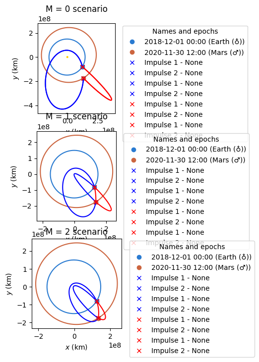
Finally, we can plot all the different scenarios from \(M=0\) up to \(M=2\) revolutions:
[6]:
from matplotlib import pyplot as plt

from poliastro.plotting import OrbitPlotter
from poliastro.plotting.orbit.backends import Matplotlib2D
[7]:
# Generate a grid of 3x1 plots
fig, axs = plt.subplots(3, 1, figsize=(8, 8))

for ith_case, M in enumerate(range(3)):
    # Plot the orbits of the Earth and Mars
    backend=Matplotlib2D(ax=axs[ith_case])
    op = OrbitPlotter(backend=backend)
    axs[ith_case].set_title(f"{M = } scenario")

    op.plot_body_orbit(Earth, EPOCH_DPT)
    op.plot_body_orbit(Mars, EPOCH_ARR)

    for ss, colorstyle in zip(
        lambert_solution_orbits(earth_departure, mars_arrival, M=M),
        colors_and_styles,
    ):
        orb_plot_traj = op.plot_maneuver(
            earth_departure, ss, color=colorstyle[0]
        )

plt.show()