Tisserand plots and applications in gravity assisted maneuvers
Spacecraft fuel is limited and thus becomes a constrain when developing interplanetary maneuvers. In order to save propellant, the mission analysis team usually benefits from the so called gravity assisted maneuvers. Although they are usually applied for increasing spacecraft velocity, they might also be used for the opposite objective. Previous kind of maneuvers are not only useful for interplanetary trips but also extremely important when designing so-called “moon tours” in Jupiter and Saturn systems.

In order to perform a preliminary gravity assist analysis, it is possible to make use of Tisserand plots. These plots illustrate how to move within different bodies for a variety of \(V_{\infty}\) and \(\alpha\), \(\alpha\) being the pump angle. Tisserand plots assume:
Perfectly circular and coplanar planet orbits. Although it is possible to include inclination within the analysis, Tisserand would no longer be 2D plots but would instead become surfaces in a three dimensional space.
Phasing is not taken into account. That means only orbits are taken into account, not rendezvous between departure and target body.
Please, note that poliastro solves ``mean orbital elements`` for Solar System bodies. Although their orbital parameters do not have great variations among time, planet orbits are assumed not to be perfectly circular or coplanar. However, Tisserand figures are still useful for quick-design gravity assisted maneuvers.
How to read the graphs
As said before, these kind of plots assume perfectly circular and coplanar orbits. Each point in a Tisserand graph is just a fly-by orbit wiht a given \(V_{\infty}\) and pump angle. That particular orbit has some energy associated, which can be computed as \(C_{Tiss}=3 - V_{\infty}^2\). The question then is, where can a spacecraft come and reach that orbit with those particular conditions?
Although Tisserand figures come in many different ways, they might be usually representing:
Periapsis VS. Apoapsis
Orbital period VS. Periapsis
Specific Energy VS. Periapsis
Let us plot a very simple Tisserand-energy kind plot for the inner planets except Mercury:
[1]:
from astropy import units as u
from matplotlib import pyplot as plt
import numpy as np

from poliastro.bodies import Venus, Earth, Mars
from poliastro.plotting.tisserand import TisserandPlotter, TisserandKind
from poliastro.plotting.util import BODY_COLORS
Notice that we imported the TisserandKind class, which will help us to indicate the kind of Tisserand plot we want to generate:
[2]:
# Show all possible Tisserand kinds
for kind in TisserandKind:
    print(f"{kind}", end="\t")
TisserandKind.APSIS TisserandKind.ENERGY TisserandKind.PERIOD
We will start by defining a TisserandPlotter instance with custom axis for a better look of the final figure. In addition, user can also make use of plot and plot_line method for representing both a collection of lines or just isolated ones.
[3]:
# Build custom axis
fig, ax = plt.subplots(1, 1, figsize=(15, 7))
ax.set_title("Energy Tisserand for Venus, Earth and Mars")
ax.set_xlabel("$R_{p} [AU]$")
ax.set_ylabel("Heliocentric Energy [km2 / s2]")
ax.set_xscale("log")
ax.set_xlim(10**-0.4, 10**0.15)
ax.set_ylim(-700, 0)

# Generate a Tisserand plotter
tp = TisserandPlotter(axes=ax, kind=TisserandKind.ENERGY)

# Plot Tisserand lines within 1km/s and 10km/s
for planet in [Venus, Earth, Mars]:
    ax = tp.plot(planet, (1, 14) * u.km / u.s, num_contours=14)

# Let us label previous figure
tp.ax.text(0.70, -650, "Venus", color=BODY_COLORS["Venus"])
tp.ax.text(0.95, -500, "Earth", color=BODY_COLORS["Earth"])
tp.ax.text(1.35, -350, "Mars", color=BODY_COLORS["Mars"])

# Plot final desired path by making use of `plot_line` method
ax = tp.plot_line(
    Venus,
    7 * u.km / u.s,
    alpha_lim=(47 * np.pi / 180, 78 * np.pi / 180),
    color="black",
)
ax = tp.plot_line(
    Mars,
    5 * u.km / u.s,
    alpha_lim=(119 * np.pi / 180, 164 * np.pi / 180),
    color="black",
)
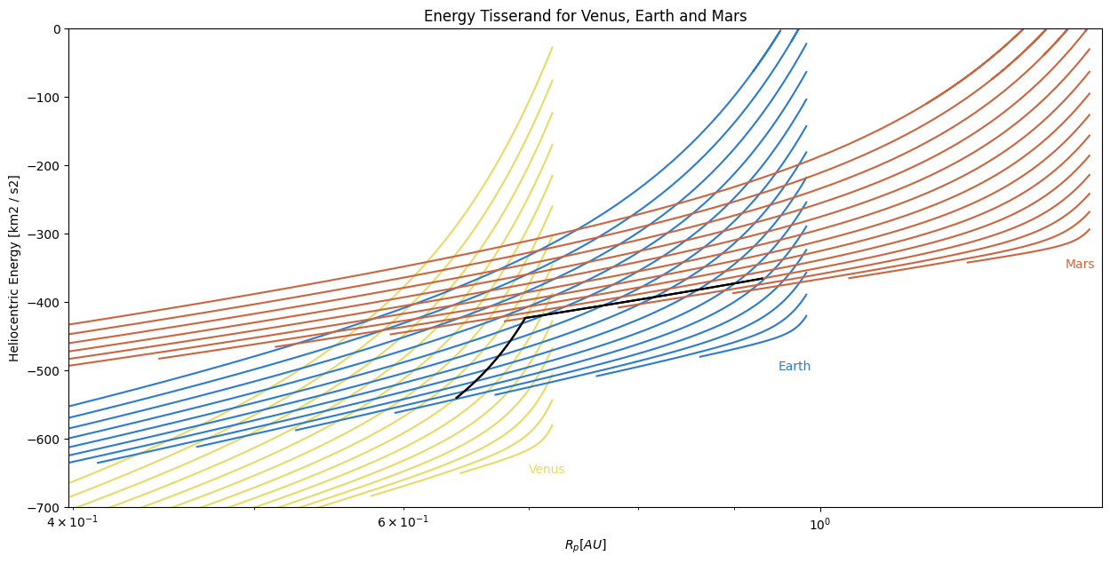
Previous black lines represent an EVME, which means Earth-Venus-Mars-Earth. Our spacecraft starts at an orbit with \(V_{\infty}=5\)km/s at Earth’s location. At this point, a trajectory shared with a \(V_{\infty}=7\)km/s for Venus is shared. This new orbit would take us to a new orbit for \(V_{\infty}=5\)km/s around Mars, which is also intercepted at some point by Earth again.
More complex tisserand graphs can be developed, for example for the whole Solar System planets. Let us check!
[4]:
# Let us import the rest of the planets
from poliastro.bodies import Mercury, Jupiter, Saturn, Uranus, Neptune

SS_BODIES_INNER = [
    Mercury,
    Venus,
    Earth,
    Mars,
]
SS_BODIES_OUTTER = [
    Jupiter,
    Saturn,
    Uranus,
    Neptune,
]
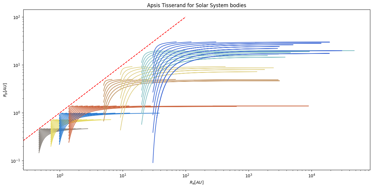
We will impose the final figure also to show a dashed red line which represents \(R_{p} = R_{a}\), meaning that orbit is perfectly circular:
[5]:
# Prellocate Tisserand figure
fig, ax = plt.subplots(1, 1, figsize=(15, 7))
ax.set_title("Apsis Tisserand for Solar System bodies")
ax.set_xlabel("$R_{a} [AU]$")
ax.set_ylabel("$R_{p} [AU]$")
ax.set_xscale("log")
ax.set_yscale("log")

# Build tisserand
tp = TisserandPlotter(axes=ax, kind=TisserandKind.APSIS)

# Show perfect circular orbits
r = np.linspace(0, 10**2) * u.AU
tp.ax.plot(r, r, linestyle="--", color="red")

# Generate lines for inner planets
for planet in SS_BODIES_INNER:
    tp.plot(planet, (1, 12) * u.km / u.s, num_contours=12)

# Generate lines for outter planets
for planet in SS_BODIES_OUTTER:
    if planet == Jupiter or planet == Saturn:
        tp.plot(planet, (1, 7) * u.km / u.s, num_contours=7)
    else:
        tp.plot(planet, (1, 5) * u.km / u.s, num_contours=10)