Revisiting Lambert’s problem in Python
The Izzo algorithm to solve the Lambert problem is available in poliastro and was implemented from this paper.
[1]:
from cycler import cycler

from matplotlib import pyplot as plt
import numpy as np

from poliastro.core import iod
from poliastro.iod import izzo
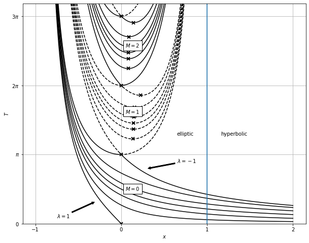
Part 1: Reproducing the original figure
[2]:
x = np.linspace(-1, 2, num=1000)
M_list = 0, 1, 2, 3
ll_list = 1, 0.9, 0.7, 0, -0.7, -0.9, -1
[3]:
fig, ax = plt.subplots(figsize=(10, 8))
ax.set_prop_cycle(
    cycler("linestyle", ["-", "--"])
    * (cycler("color", ["black"]) * len(ll_list))
)
for M in M_list:
    for ll in ll_list:
        T_x0 = np.zeros_like(x)
        for ii in range(len(x)):
            y = iod._compute_y(x[ii], ll)
            T_x0[ii] = iod._tof_equation_y(x[ii], y, 0.0, ll, M)
        if M == 0 and ll == 1:
            T_x0[x > 0] = np.nan
        elif M > 0:
            # Mask meaningless solutions
            T_x0[x > 1] = np.nan
        (l,) = ax.plot(x, T_x0)

ax.set_ylim(0, 10)

ax.set_xticks((-1, 0, 1, 2))
ax.set_yticks((0, np.pi, 2 * np.pi, 3 * np.pi))
ax.set_yticklabels(("$0$", "$\pi$", "$2 \pi$", "$3 \pi$"))

ax.vlines(1, 0, 10)
ax.text(0.65, 4.0, "elliptic")
ax.text(1.16, 4.0, "hyperbolic")

ax.text(0.05, 1.5, "$M = 0$", bbox=dict(facecolor="white"))
ax.text(0.05, 5, "$M = 1$", bbox=dict(facecolor="white"))
ax.text(0.05, 8, "$M = 2$", bbox=dict(facecolor="white"))

ax.annotate(
    "$\lambda = 1$",
    xy=(-0.3, 1),
    xytext=(-0.75, 0.25),
    arrowprops=dict(arrowstyle="simple", facecolor="black"),
)
ax.annotate(
    "$\lambda = -1$",
    xy=(0.3, 2.5),
    xytext=(0.65, 2.75),
    arrowprops=dict(arrowstyle="simple", facecolor="black"),
)

ax.grid()
ax.set_xlabel("$x$")
ax.set_ylabel("$T$")
[3]:
Text(0, 0.5, '$T$')

Part 2: Locating \(T_{min}\)
[4]:
for M in M_list:
    for ll in ll_list:
        x_T_min, T_min = iod._compute_T_min(ll, M, 10, 1e-8)
        ax.plot(x_T_min, T_min, "kx", mew=2)

fig
[4]:
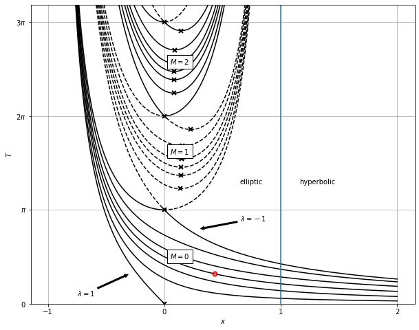
Part 3: Try out solution
[5]:
T_ref = 1
ll_ref = 0

x_ref, _ = iod._find_xy(
    ll_ref, T_ref, M=0, numiter=10, lowpath=True, rtol=1e-8
)
x_ref
[5]:
0.4334467345350424
[6]:
ax.plot(x_ref, T_ref, "o", mew=2, mec="red", mfc="none")

fig
[6]:
Part 4: Run some examples
[7]:
from astropy import units as u

from poliastro.bodies import Earth
Single revolution
[8]:
k = Earth.k
r0 = [15945.34, 0.0, 0.0] * u.km
r = [12214.83399, 10249.46731, 0.0] * u.km
tof = 76.0 * u.min

expected_va = [2.058925, 2.915956, 0.0] * u.km / u.s
expected_vb = [-3.451569, 0.910301, 0.0] * u.km / u.s

v0, v = izzo.lambert(k, r0, r, tof)
v
[8]:
$[-3.4515665,~0.91031354,~0] \; \mathrm{\frac{km}{s}}$
[9]:
k = Earth.k
r0 = [5000.0, 10000.0, 2100.0] * u.km
r = [-14600.0, 2500.0, 7000.0] * u.km
tof = 1.0 * u.h

expected_va = [-5.9925, 1.9254, 3.2456] * u.km / u.s
expected_vb = [-3.3125, -4.1966, -0.38529] * u.km / u.s

v0, v = izzo.lambert(k, r0, r, tof)
v
[9]:
$[-3.3124585,~-4.196619,~-0.38528906] \; \mathrm{\frac{km}{s}}$
Multiple revolutions
[10]:
k = Earth.k
r0 = [22592.145603, -1599.915239, -19783.950506] * u.km
r = [1922.067697, 4054.157051, -8925.727465] * u.km
tof = 10 * u.h

expected_va = [2.000652697, 0.387688615, -2.666947760] * u.km / u.s
expected_vb = [-3.79246619, -1.77707641, 6.856814395] * u.km / u.s

expected_va_l = [0.50335770, 0.61869408, -1.57176904] * u.km / u.s
expected_vb_l = [-4.18334626, -1.13262727, 6.13307091] * u.km / u.s

expected_va_r = [-2.45759553, 1.16945801, 0.43161258] * u.km / u.s
expected_vb_r = [-5.53841370, 0.01822220, 5.49641054] * u.km / u.s
[11]:
v0, v = izzo.lambert(k, r0, r, tof, M=0)
v
[11]:
$[-3.7924662,~-1.7770764,~6.8568144] \; \mathrm{\frac{km}{s}}$
[12]:
_, v_l = izzo.lambert(k, r0, r, tof, M=1, lowpath=True)
_, v_r = izzo.lambert(k, r0, r, tof, M=1, lowpath=False)
[13]:
v_l
[13]:
$[-5.5384132,~0.018222134,~5.4964102] \; \mathrm{\frac{km}{s}}$
[14]:
v_r
[14]:
$[-4.1833463,~-1.1326273,~6.1330709] \; \mathrm{\frac{km}{s}}$