Catch that asteroid!
First, we need to increase the timeout time to allow the download of data occur properly:
[1]:
from astropy.utils.data import conf

conf.dataurl
[1]:
'http://data.astropy.org/'
[2]:
conf.remote_timeout
[2]:
10.0
[3]:
conf.remote_timeout = 10000
Then, we do the rest of the imports:
[4]:
from astropy import units as u
from astropy.time import Time, TimeDelta
from astropy.coordinates import solar_system_ephemeris

solar_system_ephemeris.set("jpl")

from poliastro.bodies import Sun, Earth, Moon
from poliastro.ephem import Ephem
from poliastro.frames import Planes
from poliastro.plotting import StaticOrbitPlotter
from poliastro.plotting.misc import plot_solar_system
from poliastro.twobody import Orbit
from poliastro.util import norm, time_range

EPOCH = Time("2017-09-01 12:05:50", scale="tdb")
C_FLORENCE = "#000"
C_MOON = "#999"
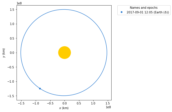
[5]:
Earth.plot(EPOCH)
[5]:
([<matplotlib.lines.Line2D at 0x7f528a8ab0a0>],
 <matplotlib.lines.Line2D at 0x7f528a8a7970>)
Our first option to retrieve the orbit of the Florence asteroid is to use Orbit.from_sbdb, which gives us the osculating elements at a certain epoch:
[6]:
florence_osc = Orbit.from_sbdb("Florence")
florence_osc
[6]:
1 x 3 AU x 22.1 deg (HeliocentricEclipticIAU76) orbit around Sun (☉) at epoch 2459800.50080073 (TDB)
However, the epoch of the result is not close to the time of the close approach we are studying:
[7]:
florence_osc.epoch.iso
[7]:
'2022-08-09 00:01:09.183'
Therefore, if we propagate this orbit to EPOCH, the results will be a bit different from the reality. Therefore, we need to find some other means.
Let’s use the Ephem.from_horizons method as an alternative, sampling over a period of 6 months:
[8]:
epochs = time_range(
    EPOCH - TimeDelta(3 * 30 * u.day), end=EPOCH + TimeDelta(3 * 30 * u.day)
)
[9]:
florence = Ephem.from_horizons("Florence", epochs, plane=Planes.EARTH_ECLIPTIC)
florence
[9]:
Ephemerides at 50 epochs from 2017-06-03 12:05:50.000 (TDB) to 2017-11-30 12:05:50.000 (TDB)
[10]:
florence.plane
[10]:
<Planes.EARTH_ECLIPTIC: 'Earth mean Ecliptic and Equinox of epoch (J2000.0)'>
And now, let’s compute the distance between Florence and the Earth at that epoch:
[11]:
earth = Ephem.from_body(Earth, epochs, plane=Planes.EARTH_ECLIPTIC)
earth
[11]:
Ephemerides at 50 epochs from 2017-06-03 12:05:50.000 (TDB) to 2017-11-30 12:05:50.000 (TDB)
[12]:
min_distance = norm(florence.rv(EPOCH)[0] - earth.rv(EPOCH)[0]) - Earth.R
min_distance.to(u.km)
[12]:
This value is consistent with what ESA says! \(7\,060\,160\) km
[13]:
abs((min_distance - 7060160 * u.km) / (7060160 * u.km)).decompose()
[13]:
[14]:
from IPython.display import HTML
HTML(
"""<blockquote class="twitter-tweet" data-lang="en"><p lang="es" dir="ltr">La <a href="https://twitter.com/esa_es">@esa_es</a> ha preparado un resumen del asteroide <a href="https://twitter.com/hashtag/Florence?src=hash">#Florence</a> 😍 <a href="https://t.co/Sk1lb7Kz0j">pic.twitter.com/Sk1lb7Kz0j</a></p>— AeroPython (@AeroPython) <a href="https://twitter.com/AeroPython/status/903197147914543105">August 31, 2017</a></blockquote>
<script src="//platform.twitter.com/widgets.js" charset="utf-8"></script>"""
)
[14]:
La @esa_es ha preparado un resumen del asteroide #Florence 😍 pic.twitter.com/Sk1lb7Kz0j
— AeroPython (@AeroPython) August 31, 2017
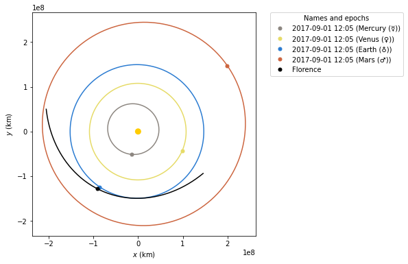
And now we can plot!
[15]:
frame = plot_solar_system(outer=False, epoch=EPOCH)
frame.plot_ephem(florence, EPOCH, label="Florence", color=C_FLORENCE)
[15]:
([<matplotlib.lines.Line2D at 0x7f52867851f0>],
 <matplotlib.lines.Line2D at 0x7f5286785e80>)
Finally, we are going to visualize the orbit of Florence with respect to the Earth. For that, we set a narrower time range, and specify that we want to retrieve the ephemerides with respect to our planet:
[16]:
epochs = time_range(
    EPOCH - TimeDelta(5 * u.day), end=EPOCH + TimeDelta(5 * u.day)
)
[17]:
florence_e = Ephem.from_horizons("Florence", epochs, attractor=Earth)
florence_e
[17]:
Ephemerides at 50 epochs from 2017-08-27 12:05:50.000 (TDB) to 2017-09-06 12:05:50.000 (TDB)
We now retrieve the ephemerides of the Moon, which are given directly in GCRS:
[18]:
moon = Ephem.from_body(Moon, epochs, attractor=Earth)
moon
[18]:
Ephemerides at 50 epochs from 2017-08-27 12:05:50.000 (TDB) to 2017-09-06 12:05:50.000 (TDB)
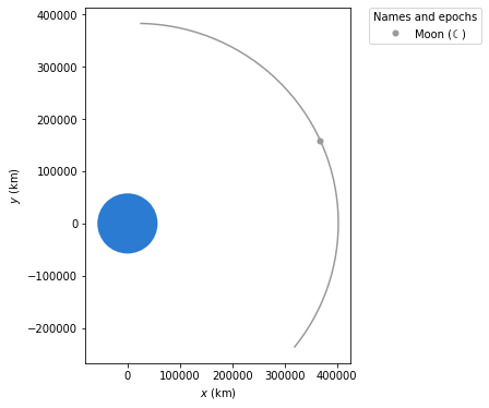
[19]:
plotter = StaticOrbitPlotter()
plotter.set_attractor(Earth)
plotter.set_body_frame(Moon)
plotter.plot_ephem(moon, EPOCH, label=Moon, color=C_MOON)
[19]:
([<matplotlib.lines.Line2D at 0x7f52865b65b0>],
 <matplotlib.lines.Line2D at 0x7f52865b6820>)
And now, the glorious final plot:
[20]:
from matplotlib import pyplot as plt

frame = StaticOrbitPlotter()

frame.set_attractor(Earth)
frame.set_orbit_frame(Orbit.from_ephem(Earth, florence_e, EPOCH))

frame.plot_ephem(florence_e, EPOCH, label="Florence", color=C_FLORENCE)
frame.plot_ephem(moon, EPOCH, label=Moon, color=C_MOON)
[20]:
([<matplotlib.lines.Line2D at 0x7f5284d2a5b0>],
 <matplotlib.lines.Line2D at 0x7f5284d23fd0>)
