Detecting Events
It is a well-known fact that launching a satellite is a captial-intensive and fuel-exhaustive process. Moreover, maintaining high accuracy and precision in any satellite orbit analysis is paramount to be able to comprehend helpful information from them.
Detecing some peculiar phenomena associated with satellites, which we call “events”, could provide beneficial insights about their orbit dynamics for further treatment. While some could provide critical scientific information and help us formulate efficient space strategies and policies, the potentially disastrous ones, like satellite collisions, could help us take further steps to prevent such contingencies.
This notebook gives a glimpse of poliastro’s event detection capabilities. The procedure to track an event during an orbit’s propagation is fairly simple:
Instantiate the desired event class/classes.
Pass the
Eventobject(s) as an argument toCowellPropagator.Detect events! Optionally, the
terminalanddirectionattributes can be set as required.
[1]:
# Imports
import numpy as np
from numpy.linalg import norm
import matplotlib.pyplot as plt

import astropy
import astropy.units as u
from astropy.time import Time
from astropy.coordinates import (
    CartesianRepresentation,
    get_body_barycentric_posvel,
)

from poliastro.bodies import Earth, Sun

from poliastro.twobody.events import (
    AltitudeCrossEvent,
    LatitudeCrossEvent,
    NodeCrossEvent,
    PenumbraEvent,
    UmbraEvent,
)
from poliastro.twobody.orbit import Orbit
from poliastro.twobody.propagation import CowellPropagator
from poliastro.twobody.sampling import EpochsArray

from poliastro.util import time_range
Altitude Crossing Event
Let’s define some natural perturbation conditions for our orbit so that its altitude decreases with time.
[2]:
from poliastro.constants import H0_earth, rho0_earth
from poliastro.core.perturbations import atmospheric_drag_exponential
from poliastro.core.propagation import func_twobody

R = Earth.R.to_value(u.km)

# Parameters of the body
C_D = 2.2  # Dimensionless (any value would do)
A_over_m = ((np.pi / 4.0) * (u.m**2) / (100 * u.kg)).to_value(
    u.km**2 / u.kg
)  # km^2/kg

# Parameters of the atmosphere
rho0 = rho0_earth.to_value(u.kg / u.km**3)  # kg/km^3
H0 = H0_earth.to_value(u.km)  # km


def f(t0, u_, k):
    du_kep = func_twobody(t0, u_, k)
    ax, ay, az = atmospheric_drag_exponential(
        t0, u_, k, R=R, C_D=C_D, A_over_m=A_over_m, H0=H0, rho0=rho0
    )
    du_ad = np.array([0, 0, 0, ax, ay, az])
    return du_kep + du_ad
We shall use the CowellPropagator with the above perturbating conditions and pass the events we want to keep track of, in this case only the AltitudeCrossEvent.
[3]:
tofs = np.arange(0, 2400, 100) << u.s
orbit = Orbit.circular(Earth, 150 * u.km)

# Define a threshold altitude for crossing.
thresh_alt = 50  # in km
altitude_cross_event = AltitudeCrossEvent(thresh_alt, R)  # Set up the event.
events = [altitude_cross_event]

method = CowellPropagator(events=events, f=f)
rr, _ = orbit.to_ephem(
    EpochsArray(orbit.epoch + tofs, method=method),
).rv()

print(
    f"The threshold altitude was crossed {altitude_cross_event.last_t} after the orbit's epoch."
)
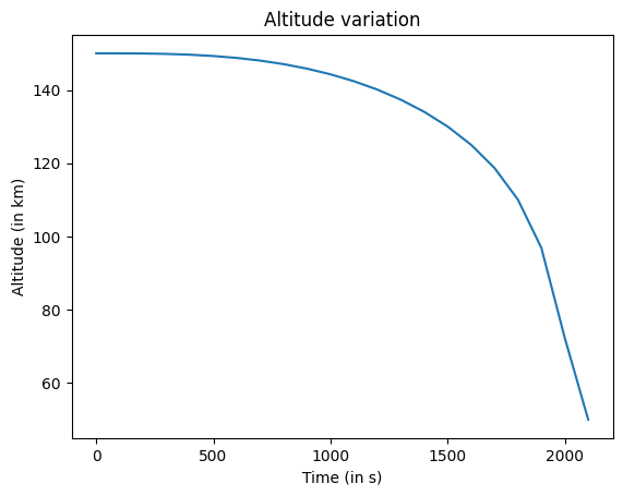
The threshold altitude was crossed 2063.6700936204934 s after the orbit's epoch.
Let’s see how did the orbit’s altitude vary with time:
[4]:
altitudes = np.apply_along_axis(
    norm, 1, (rr << u.km).value
) - Earth.R.to_value(u.km)
plt.plot(tofs[: len(rr)].to_value(u.s), altitudes)
plt.title("Altitude variation")
plt.ylabel("Altitude (in km)")
plt.xlabel("Time (in s)")
[4]:
Text(0.5, 0, 'Time (in s)')
Refer to the API documentation of the events to check the default values for terminal and direction and change it as required.
Latitude Crossing Event
Similar to the AltitudeCrossEvent, just pass the threshold latitude while instantiating the event.
[5]:
orbit = Orbit.from_classical(
    Earth,
    6900 << u.km,
    0.75 << u.one,
    45 << u.deg,
    0 << u.deg,
    0 << u.deg,
    130 << u.deg,
)
[6]:
thresh_lat = 35 << u.deg
latitude_cross_event = LatitudeCrossEvent(orbit, thresh_lat, terminal=True)
events = [latitude_cross_event]

tofs = np.arange(0, 20 * orbit.period.to_value(u.s), 150) << u.s
method = CowellPropagator(events=events)
rr, _ = orbit.to_ephem(EpochsArray(orbit.epoch + tofs, method=method)).rv()
print(
    f"The threshold latitude was crossed {latitude_cross_event.last_t} s after the orbit's epoch"
)
The threshold latitude was crossed 5225.7148541757415 s s after the orbit's epoch
Let’s plot the latitude varying with time:
[7]:
from poliastro.core.spheroid_location import cartesian_to_ellipsoidal

latitudes = []
for r in rr:
    position_on_body = (r / norm(r)) * Earth.R
    _, lat, _ = cartesian_to_ellipsoidal(
        Earth.R, Earth.R_polar, *position_on_body
    )
    latitudes.append(np.rad2deg(lat))
plt.plot(tofs[: len(rr)].to_value(u.s), latitudes)
plt.title("Latitude variation")
plt.ylabel("Latitude (in degrees)")
plt.xlabel("Time (in days)")
[7]:
Text(0.5, 0, 'Time (in days)')
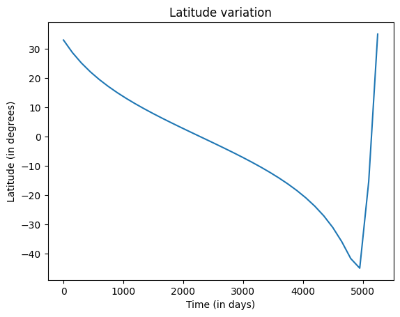
The orbit’s latitude would not change after the event was detected since we had set terminal=True.
Since the attractor is Earth, we could use GroundtrackPlotter for showing the groundtrack of the orbit on Earth.
[8]:
from poliastro.earth import EarthSatellite
from poliastro.earth.plotting import GroundtrackPlotter
from poliastro.plotting import OrbitPlotter

es = EarthSatellite(orbit, None)

# Show the groundtrack plot from
t_span = time_range(orbit.epoch, end=orbit.epoch + latitude_cross_event.last_t)

# Generate ground track plotting instance.
gp = GroundtrackPlotter()
gp.update_layout(title="Latitude Crossing")

# Plot the above-defined earth satellite.
gp.plot(
    es,
    t_span,
    label="Orbit",
    color="red",
    marker={
        "size": 10,
        "symbol": "triangle-right",
        "line": {"width": 1, "color": "black"},
    },
)
Viewing it in the orthographic projection mode,
[9]:
gp.update_geos(projection_type="orthographic")
gp.fig.show()
and voila! The groundtrack terminates almost at the 35 degree latitude mark.
Eclipse Event
Users can detect umbra/penumbra crossings using the UmbraEvent and PenumbraEvent event classes, respectively. As seen from the above examples, the procedure doesn’t change much.
[10]:
from poliastro.core.events import eclipse_function

attractor = Earth
tof = 2 * u.d
# Classical orbital elements
coe = (
    7000.137 * u.km,
    0.009 * u.one,
    87.0 * u.deg,
    20.0 * u.deg,
    10.0 * u.deg,
    0 * u.deg,
)
orbit = Orbit.from_classical(attractor, *coe)
Let’s search for umbra crossings.
[11]:
umbra_event = UmbraEvent(orbit, terminal=True)
events = [umbra_event]

tofs = np.arange(0, 600, 30) << u.s
method = CowellPropagator(events=events)
rr, vv = orbit.to_ephem(EpochsArray(orbit.epoch + tofs, method=method)).rv()
print(
    f"The umbral shadow entry time was {umbra_event.last_t} after the orbit's epoch"
)
The umbral shadow entry time was 524.7274279607626 s after the orbit's epoch
Note: Even though the eclipse events UmbraEvent and PenumbraEvent take the Orbit as input, they are not used in propagation but used only to access some helpful attributes of the orbit.
Let us plot the eclipse functions’ variation with time.
[12]:
k = Earth.k.to_value(u.km**3 / u.s**2)
R_sec = Sun.R.to_value(u.km)
R_pri = Earth.R.to_value(u.km)
# Position vector of Sun wrt Solar System Barycenter
r_sec_ssb = get_body_barycentric_posvel("Sun", orbit.epoch)[0]
r_pri_ssb = get_body_barycentric_posvel("Earth", orbit.epoch)[0]

r_sec = ((r_sec_ssb - r_pri_ssb).xyz << u.km).value

rr = (rr << u.km).value
vv = (vv << u.km / u.s).value

eclipses = []  # List to store values of eclipse_function.
for i in range(len(rr)):
    r = rr[i]
    v = vv[i]
    eclipse = eclipse_function(k, np.hstack((r, v)), r_sec, R_sec, R_pri)
    eclipses.append(eclipse)

plt.xlabel("Time (s)")
plt.ylabel("Eclipse function")
plt.title("Eclipse function vs time")
plt.plot(tofs[: len(rr)].to_value(u.s), eclipses)
[12]:
[<matplotlib.lines.Line2D at 0x7f4bb7a9b850>]
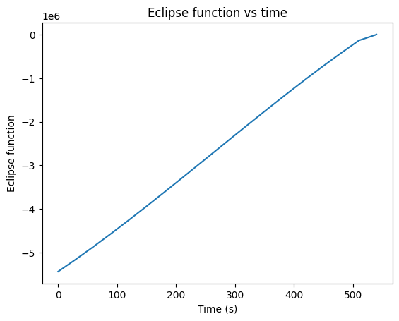
For simplicity, here we compute the position vector of the primary and the secondary body only once, at the orbit epoch. However, the eclipse events internally recompute the position vectors at each desired instant.
We could get some geometrical insights by plotting the orbit:
[13]:
# Plot `Earth` at the instant of event occurence.
Earth.plot(
    orbit.epoch.tdb + umbra_event.last_t,
    label="Earth position at event instance",
)

plotter = OrbitPlotter()

plotter.plot(orbit)
plotter.set_orbit_frame(orbit)

# Convert satellite coordinates to a `CartesianRepresentation` object.
coords = CartesianRepresentation(
    rr[:, 0] << u.km, rr[:, 1] << u.km, rr[:, 2] << u.km
)
plotter.plot_trajectory(coords, color="orange")
[13]:
(<matplotlib.lines.Line2D at 0x7f4bb9b877f0>, None)
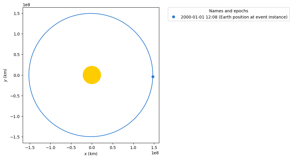
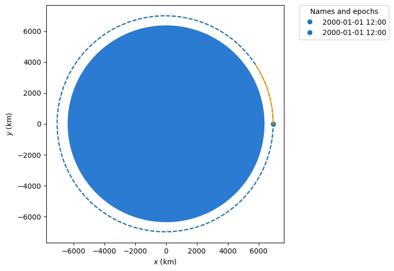
It seems our satellite is exiting the umbra region, as is evident from the orange colored trajectory!
Node Cross Event
This event detector aims to check for ascending and descending node crossings. Note that it could yield inaccurate results if the orbit is near-equatorial.
[14]:
r = [-3182930.668, 94242.56, -85767.257] << u.km
v = [505.848, 942.781, 7435.922] << u.km / u.s
orbit = Orbit.from_vectors(Earth, r, v)
As a sanity check, let’s check the orbit’s inclination to ensure it is not near-zero:
[15]:
print(orbit.inc)
1.699055905117056 rad
Indeed, it isn’t!
[16]:
node_event = NodeCrossEvent(terminal=True)
events = [node_event]

tofs = [0.01, 0.1, 0.5, 0.8, 1, 3, 5, 6, 10, 11, 12, 13, 14, 15] << u.s
method = CowellPropagator(events=events)
rr, vv = orbit.to_ephem(EpochsArray(orbit.epoch + tofs, method=method)).rv()

print(f"The nodal cross time was {node_event.last_t} after the orbit's epoch")
The nodal cross time was 11.534179218118878 s after the orbit's epoch
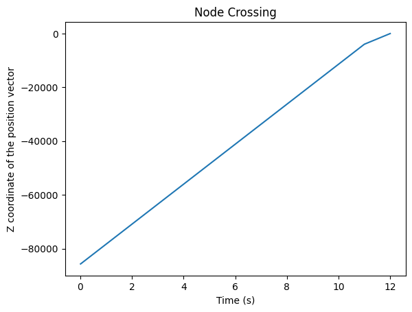
The plot below shows us the variation of the z coordinate of the orbit’s position vector with time:
[17]:
z_coords = [r[-1].to_value(u.km) for r in rr]
plt.xlabel("Time (s)")
plt.ylabel("Z coordinate of the position vector")
plt.title("Node Crossing")
plt.plot(tofs[: len(rr)].to_value(u.s), z_coords)
[17]:
[<matplotlib.lines.Line2D at 0x7f4bb943a3a0>]
We could do the same plotting done in LatitudeCrossEvent to check for equatorial crossings:
[18]:
es = EarthSatellite(orbit, None)

# Show the groundtrack plot from
t_span = time_range(
    orbit.epoch - 1.5 * u.h, end=orbit.epoch + node_event.last_t
)

# Generate ground track plotting instance.
gp = GroundtrackPlotter()
gp.update_layout(title="Node Crossing")

# Plot the above-defined earth satellite.
gp.plot(
    es,
    t_span,
    label="Orbit",
    color="red",
    marker={
        "size": 10,
        "symbol": "triangle-right",
        "line": {"width": 1, "color": "black"},
    },
)
[19]:
gp.update_geos(projection_type="orthographic")
gp.fig.show()
Indeed, we can observe that it’s an ascending node crossing! If we want to only detect either of the two crossings, the direction attribute is at our disposal!
Multiple Event Detection
If we would like to track multiple events while propagating an orbit, we just need to add the concerned events inside events. Below, we show the case where NodeCrossEvent and LatitudeCrossEvent events are to be detected.
[20]:
# NodeCrossEvent is detected earlier than the LatitudeCrossEvent.
r = [-6142438.668, 3492467.56, -25767.257] << u.km
v = [505.848, 942.781, 7435.922] << u.km / u.s
orbit = Orbit.from_vectors(Earth, r, v)

# Node Cross event
node_cross_event = NodeCrossEvent(terminal=True)
# Latitude event
thresh_lat = 60 * u.deg
latitude_cross_event = LatitudeCrossEvent(orbit, thresh_lat, terminal=True)

events = [node_cross_event, latitude_cross_event]

tofs = [1, 2, 4, 6, 8, 10, 12] << u.s
method = CowellPropagator(events=events)
rr, vv = orbit.to_ephem(EpochsArray(orbit.epoch + tofs, method=method)).rv()

print(f"Node cross event termination time: {node_cross_event.last_t} s")
print(
    f"Latitude cross event termination time: {latitude_cross_event.last_t} s"
)
Node cross event termination time: 3.46524035620598 s s
Latitude cross event termination time: 8.861147813829435 s s
When detecting multiple events, the propagation stops as soon as any event, with the terminal property set to True, is detected.